Brownian Motion: Order from Chaos
Brownian Motion
Brownian motion can be defined as the random motion of particles in a liquid or gas caused by the bombardment from molecules in the containing medium. Have you ever looked at dust particles in the sunlight shining through a window? They appear to move about randomly, even defying gravity. This is an example of Brownian motion in which the dust particles are bombarded on all sides by gas molecules in the air. Other examples of Brownian motion include the motion of grains of pollen on the surface of still water, the diffusion of air pollutants, the diffusion of a drop of ink in hot water, and the motion of "holes" of electrical charge in semiconductors, just to mention a few.
There are many Web-based simulations that illustrate Brownian motion. Some are interactive, some make use of Matlab, some are downloadable, and most provide animations showing the random motion of a particle being bombarded by molecules. The author of this lesson found only one physical Brownian motion demonstration, presented by Saint Mary's University in Halifax, NS. It uses a plastic chip as the particle being bombarded and small metal beads representing the bombarding molecules. No discussion is presented on how the beads were set into motion, and the demonstration was entirely qualitative, with no suggestions for performing a quantitative lab of any kind with the apparatus.
Here, we present a quantitative Brownian motion lab using steel balls as the molecules and a small, round plastic disk as the particle under bombardment. A separate pdf file that accompanies this lesson provides details on how the apparatus was constructed. The main component of the apparatus is an orbital shaker. This shaker provides the energy to keep the steel balls moving. Check out the accompanying pdf file for additional details on construction of the apparatus. The cost of the orbital shaker was less than $80, the cost of materials was about $25, and the construction time was about an hour.
The Experiment Design
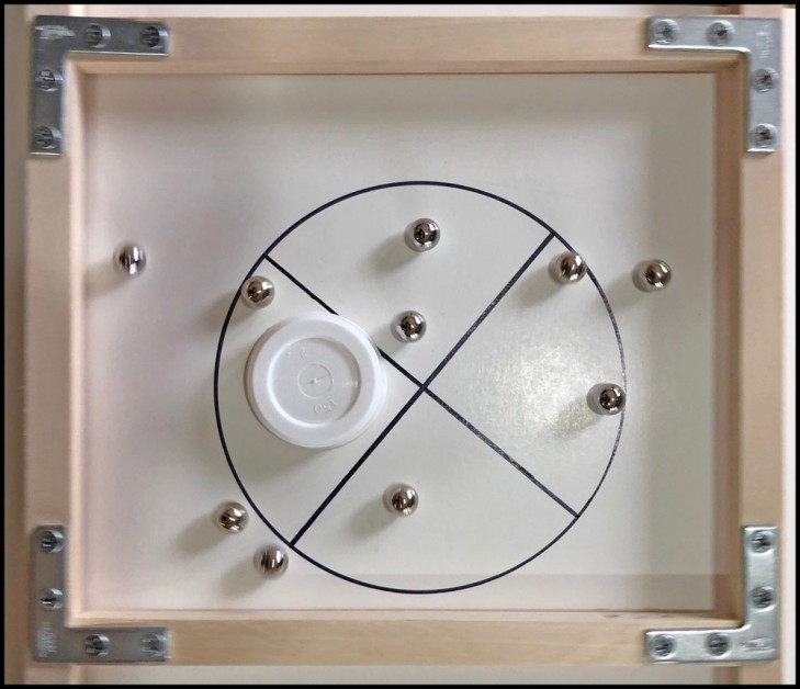
Figure 1 shows a birdseye view of the apparatus. The wood frame vibrates back-and-forth at 210 cycles per minute in sync with the orbital shaker (not shown in the picture), providing the energy to keep the steel balls in motion. Ten steel balls representing the bombarding molecules are rolling on a piece of foam board. The steel balls are 3/8" in diameter. A small hollow plastic disk is the particle that is being bombarded from the random impacts of the steel balls. This disk must be light enough so that the steel ball impacts will move it well. A circle of diameter 4.75" and crosshairs have been drawn on the foam board.
The video below shows the Brownian motion simulator in action. Note that the foam board with the circle and crosshairs, on which the steel balls and disk are located, is at rest. The wood frame, however, is fixed to the orbital shaker to provide impacts that keep the steel balls moving about randomly.
The Student Task
The task for the student is to determine a distribution for the amount of time t required for the disk to move from the center of the circle until any part of the disk crosses the circumference of the circle. We say distribution of times, as time will vary significantly from trial to trial. Distributions are commonly shown by the use of histograms. A typical histogram might indicate the number of times that t is between 0 and 5 seconds, between 5 and 10 seconds, between 10 and 15 seconds, etc.
When data is collected for histograms, it is advisable to conduct a fairly large number of trials--between 80 and 100 is recommended. Using a stop watch to collect and then record such data would be rather tedious! PocketLab Voyager's tactile sensor to the rescue!
With the steel balls moving randomly about, place the disk at the center of the circle on the foam board and give a quick, firm tap of the tactile sensor with your forefinger. When any part of the disk crosses the circumference of the circle, tap the tactile sensor again, and quickly move the disk back to the center of the circle. Repeat this process for 15 minutes. You will wind up with on the order of 100 spikes on the tactile sensor versus time graph. Figure 2 shows an example Excel graph with these spikes. The time between adjacent spikes corresponds to the time required for the disk to move from the center of the circle until its edge just crosses the circle.
Here is where the student can hone his or her Excel skills! A careful analysis and Excel manipulation of the tactile sensor csv file produced by the PocketLab app will allow producing a histogram. (Hint: Manipulation will include several sorts of the data, removal of unwanted data, copying data values only from one sheet to another in the Excel workbook, and final creation of the histogram statistics chart.)
Typical Experiment Results and Discussion
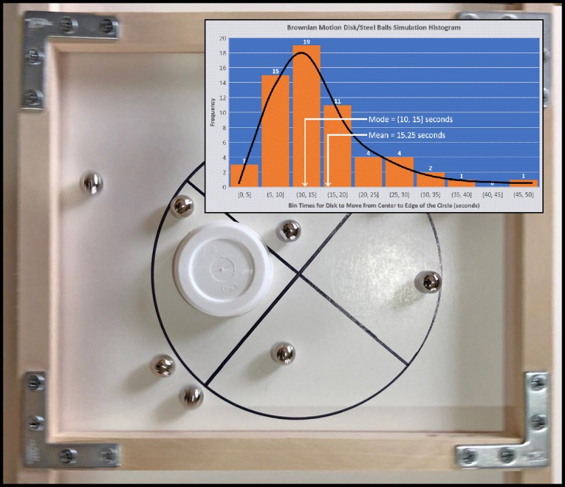
Figure 3 shows the author's histogram for a run with 10 steel balls. The black curve was drawn over the histogram to emphasize the general shape of the distribution. This curve was post drawn on the histogram by using the curve drawing feature of PowerPoint.
This histogram speaks to the title of this lesson "Brownian Motion: Order from Chaos". The histogram shows that in spite of the chaotic random collisions of the steel balls with the disk, there is a definite pattern that emerges in the time for the disk to move from the center of the circle to the edge of the circle. The curve is not a bell-shaped normal distribution. It shows that the probability (frequency) is relatively low for times from 0 to 5 seconds. It further shows that the peak interval (the mode) for these times is between 10 and 15 seconds. There is a long tail on the right indicating that the probabilities for higher and higher times quickly drops. Intuition suggests that the tail should extend forever to the right, but with extremely small probabilities. The long tail contains the "outliers"--those trials where you may have thought that the disk would never reach the edge of the circle!
With the bulk of the trials on the left, statisticians say that the distribution is skewed to the left. Our distribution differs from the bell-shaped (normal) distribution in at least two major ways. First, the normal distribution is symmetric--i.e., has the same shape to the left and right of the mode. Our distribution is asymmetric since the shape of the curve is different to the left and right of the mode. Secondly, the normal distribution has infinite long tails on both the left an right. Our distribution only has a tail on the right. There cannot possibly be a tail on the left as our measured times cannot be negative. The lowest possible time would be zero. Maybe we should say very small but not zero--even light would take a finite positive amount of time to travel from the center to the edge of the disk!
Lastly, the mode and mean were noted on our histogram. For our distribution the mean is higher than the mode, because of the existence of outliers on the far right.
Optional Investigation
Does the number of molecules affect the shape of the distribution? A good way to check this out would be to do runs with five steel balls instead of 10, or 20 steel balls instead of 10.
Final Comments
This has been an interdisciplinary investigation. Brownian motion is central to the study of chemistry and physics as it provides evidence for the existence of atoms that cannot be seen, but whose effects can be seen on the motion of larger particles. This lesson has also investigated terms related to the study of statistics and probability--histograms, distributions, symmetric, asymmetric, skew, mode, and mean. Finally, students learned that a tactile sensor can be used to aid in timing events when data from this sensor is properly analyzed with spreadsheet software.
An Additional Quantitative Lesson Dealing with a Steel Ball Model