Lissajous Introduction
Lissajous patterns have fascinated physics students for decades. They are commonly observed on oscilloscopes by applying simple harmonic functions with different frequencies to the vertical and horizontal inputs. Three examples are shown in Figure 1. From left to right, the frequency ratios are 1:2, 2:3, and 3:4. These Lissajous patterns were created by use of the parametric equation section of The Grapher software written by the author of this lesson. You are welcome to use this software for graphing prepared or custom functions, polar equations, and parametric equations.
The graphs of Figure 1 can only be obtained in driven oscillations, meaning that there is no damping of the oscillations as time goes on. The parametric equations for Lissajous patterns of this type take on the form:
x = A sin(at + delta)
y = B sin(bt).
In these equations, t is time, A and B are the amplitudes of the oscillations, a and b are the frequencies, and delta is the phase difference between them. In many real-world situations, however, the amplitudes decrease with time due to a variety of non-conservative forces such as friction. For example, the periodic motion of physical pendulums experiences damping with the passage of time. The above pair of parametric equations can easily be modified to include damping. If we assume that the damping is negative exponential, then the equations take on the form:
x = A sin(at + delta) exp(-dt)
y = B sin(bt) exp(-dt).
In these parametric equations, the exponential damping factor d has been included, with this factor assumed the same for both the x and y oscillations. This lesson will involve the study of damped Lissajous patterns, a subject that is generally not discussed much in physics classes. Never-the-less, such a study is quite interesting and well worth the time spent.
The Damped Lissajous Experiment Setup
Figure 2 shows the setup for our damped Lissajous lab. The damped oscillations are provided by a pair of pendulums, each approximately two meters in length. In fact, the pendulums can be a couple of inches different in length, as we want the periods to be slightly different. It is best to have pendulums that are at least two meters in length, as this provides for longer periods that plot better with the PocketLab/Phyphox combination. The pendulums are constructed from four meter sticks and are suspended from the ceiling in such a way that their planes of oscillation are perpendicular to one another. A piece of 6" x 8" card stock is taped to the bottom of each pendulum. The purpose of the card stock is to provide a white surface from which the Voyager IR rangefinders can bounce their beams. A pair of perpendicular Voyagers are arranged with their rangefinders facing the card stock on the pendulums. The Voyagers are about 18" from the pendulums when the pendulums are at rest. The Voyagers are connected via BLE (Bluetooth Low Energy) to a device running Phyphox software. With the Lissajous Activity experiment running in Phyphox, the pendulums are released from rest about 4" from their respective Voyagers. Phyphox records and displays the resultant Lissajous figure while the pendulums swing back and forth with damping.
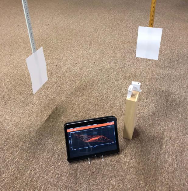
The 0.5 minute video below shows a typical data collection run of this experiment.
Results and Comparison to Theory
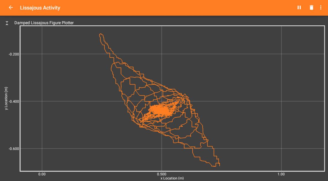
Figure 3 shows a typical Lissajous pattern plotted in Phyphox for this experiment. Note the concentration of points near the "center" of the pattern. Does this result agree with that predicted from theory?
Let's consider the following set of parametric equations:
x = sin(1.07t + π/2) exp(-0.03t); y = sin(t) exp(-0.03t).
A phase difference of π is used. Note that changing the phase difference can result in significant differences in the resultant pattern. This equation implies a 7% difference between the x and y frequencies. This was found by measuring the x and y periods with a stopwatch. The damping factor was set to 0.03. When this equation is graphed with the author's The Grapher software, the resultant graph appears as shown in Figure 4. There are clear similarities between our experimental results and theory, including the concentration of data points near the center of the figure. This concentration of points is obtained when the oscillations have been damped significantly. Here is exactly how you would key in these parametric equations using The Grapher software:
x=sin(1.07*t+PI)*exp(-0.03*t);|y=sin(t)*exp(-0.03*t)
Phyphox Software
Phyphox (physical phone experiments) is a free app developed at the 2nd Institute of Physics of the RWTH Aachen University in Germany. The author of this lesson has been working with a pre-release Android version of this app. It supports BLE (Bluetooth Low Energy) technology to transfer data from multiple Voyagers to the Phyphox app. Since then, a public Android version of the Phyphox app has been made available.
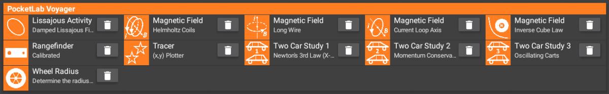
The experiment of this lesson is in a file named Lissajous.phyphox and accompanies this lesson. This file can then be opened in Phyphox and will appear in the PocketLab Voyager category of the main screen, similar to that in Figure 5.
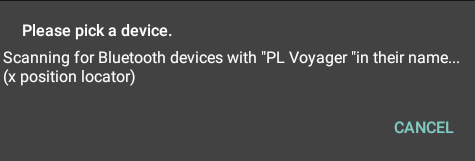
Both Voyagers should initially be turned off. The first screen that you will see after selecting the Lissajous experiment from the menu contains the message shown in Figure 6. In response to this message you should turn on the Voyager labeled X. "PL Voyager" will appear in the message. Click on "PL Voyager" and a message will tell you that Bluetooth is connecting to the device. Another message similar to that of Figure 6 will then appear, and your response to this message should be to turn on the Voyager labeled Y. When both connections are complete, you can start data collection whenever you are ready with the pulsating triangle in the upper right corner of the screen.
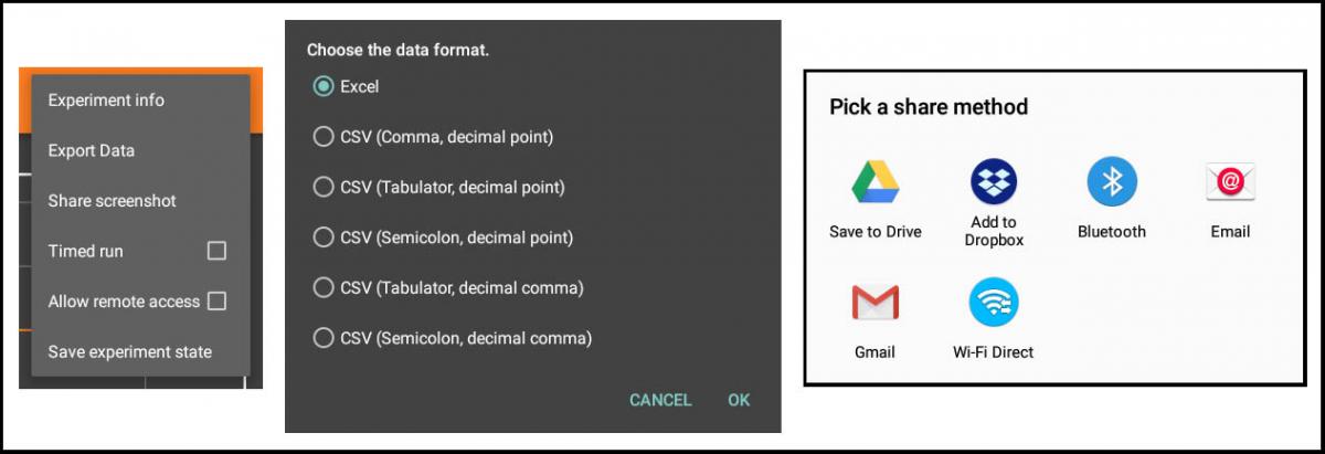
If you want to export the collected data , all you need to do is click the ellipsis in the upper right corner of the screen and select Export Data from the drop-down menu. You can then choose the desired data format (Excel, CSV) and pick a method for sharing the data (Google Drive, Email, etc.). See Figure 7.